
import matplotlib.pylab as pylab
# forces plots to appear in the ipython notebook
%matplotlib inline
from scipy.integrate import odeint
from pylab import plot,xlabel,ylabel,title,legend,figure,subplots
from pylab import cos, pi, arange, sqrt, pi, array, arrayاین سیستم به عنوان یک تابع پایتون MassSpringDamper نشون دادم که پارامترها را میتونیم به راحتی با تغییر متغیرهای این تابع تنظیم کردdef MassSpringDamper(state,t):
'''
k=spring constant, Newtons per metre
m=mass, Kilograms
c=dampign coefficient, Newton*second / meter
for a mass,spring
xdd = ((-k*x)/m) + g
for a mass, spring, damper
xdd = -k*x/m -c*xd-g
for a mass, spring, dmaper with forcing function
xdd = -k*x/m -c*xd-g + cos(4*t-pi/4)
'''
k=124e3 # spring constant, kN/m
m=64.2 # mass, Kg
c=3 # damping coefficient
# unpack the state vector
x,xd = state # displacement,x and velocity x'
g = 9.8 # metres per second**2
# compute acceleration xdd = x''
omega = 1.0 # frequency
phi = 0.0 # phase shift
A = 5.0 # amplitude
xdd = -k*x/m -c*xd-g + A*cos(2*pi*omega*t - phi)
return [xd, xdd]
شرایط تغییر مکان و سرعت اولیه در حالت متغیر 0 تعریف شده
state0 = [0.0, 1.2] #initial conditions [x0 , v0] [m, m/sec]
ti = 0.0 # initial time
tf = 4.0 # final time
step = 0.001 # step
t = arange(ti, tf, step)
state = odeint(MassSpringDamper, state0, t)
x = array(state[:,[0]])
xd = array(state[:,[1]
حل یک معادله دیفرانسیل به اندازه کافی چالش برانگیز ه
# Plotting displacement and velocity
pylab.rcParams['figure.figsize'] = (15, 12)
pylab.rcParams['font.size'] = 18
fig, ax1 = pylab.subplots()
ax2 = ax1.twinx()
ax1.plot(t,x*1e3,'b',label = r'$x (mm)$', linewidth=2.0)
ax2.plot(t,xd,'g--',label = r'$\dot{x} (m/sec)$', linewidth=2.0)
ax2.legend(loc='lower right')
ax1.legend()
ax1.set_xlabel('time , sec')
ax1.set_ylabel('disp (mm)',color='b')
ax2.set_ylabel('velocity (m/s)',color='g')
pylab.title('Mass-Spring System with $V_0=1.2 \frac{m}{s}$ and $\delta_{max}=22.9mm$')
pylab.grid()
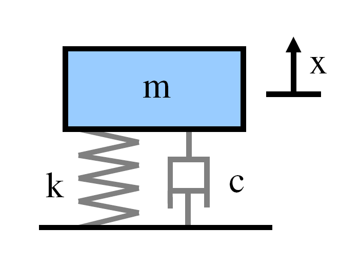
ارتعاش ازاد یک سیستم جرم فنر-دمپر
این ارتعاش آزاد یک سیستم ساده جرم فنر-دمپر را شبیه سازی می کنه به طور خاص، نحوه پاسخ سیستم به شرایط اولیه غیر صفر را بررسی میکنم
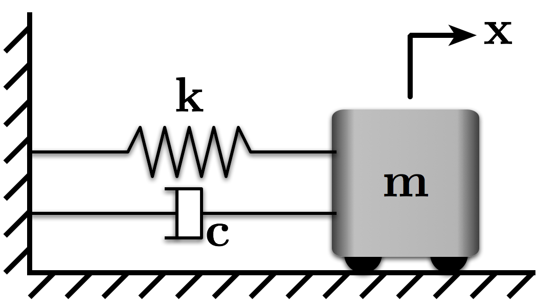
معادله حرکت سیستم به صورت زیر است:
$\quad m \ddot{x} + c \dot{x} + kx = 0$
همچنین میتونم این معادله را بر حسب نسبت میرایی، ζ و فرکانس طبیعی ω بنویسم
$\quad \ddot{x} + 2\zeta\omega_n\dot{x} + \omega_n^2x = 0$
. راه حل برای مورد کم میرایی این است:
$\quad x(t) = e^{-\zeta\omega_nt}\left(a_1 e^{i \omega_d t} + a_2 e ^{-i \omega_d t}\right)$
یا
$\quad x(t) = e^{-\zeta\omega_nt}\left(b_1 \cos{\omega_d t} + b_2 \sin{\omega_d t}\right)$
برای استفاده از این معادله باید a1 و a2 یا b1 و b2 را با استفاده از شرایط اولیه حل کنیم. در اینجا، اجازه دهید از شکل گناه/کسینوس استفاده کنیم. با حل معادله سرعت اولیه عمومی،$\dot{x} = v_0$، و یک جابجایی اولیه عمومی،$x = x_0$، متوجه میشویم:
$\quad x(t) = e^{-\zeta\omega_nt}\left(x_0 \cos{\omega_d t} + \frac{\zeta \omega_n x_0 + v_0}{\omega_d} \sin{\omega_d t}\right)$
numpy را به عنوان np وارد کنید
import numpy as np # Grab all of the NumPy functions with nickname np
%matplotlib inline
# Import the plotting functions
import matplotlib.pyplot as plt
# Define the System Parameters
m = 1.0 # kg
k = (2.0 * np.pi)**2. # N/m (Selected to give an undamped natrual frequency of 1Hz)
wn = np.sqrt(k/m) # Natural Frequency (rad/s)
z = 0.1 # Define a desired damping ratio
c = 2*z*wn*m # calculate the damping coeff. to create it (N/(m/s))
wd = wn*np.sqrt(1 - z**2) # Damped natural frequency (rad/s)
# Set up simulation parameters
t = np.linspace(0, 5, 501) # Time for simulation, 0-5s with 501 points in-between
# Define the initial conditions x(0) = 1 and x_dot(0) = 0
x0 = np.array([-1.0, 0.0])
# Define x(t)
x = np.exp(-z*wn*t)*(x0[0]*np.cos(wd*t) + (z*wn*x0[0] + x0[1])/wd * np.sin(wd*t))
# # Make the figure pretty, then plot the results
# # "pretty" parameters selected based on pdf output, not screen output
# # Many of these setting could also be made default by the .matplotlibrc file
# Set the plot size - 3x2 aspect ratio is best
fig = plt.figure(figsize=(6, 4))
ax = plt.gca()
plt.subplots_adjust(bottom=0.17, left=0.17, top=0.96, right=0.96)
# Change the axis units to serif
plt.setp(ax.get_ymajorticklabels(),family='serif',fontsize=18)
plt.setp(ax.get_xmajorticklabels(),family='serif',fontsize=18)
ax.spines['right'].set_color('none')
ax.spines['top'].set_color('none')
ax.xaxis.set_ticks_position('bottom')
ax.yaxis.set_ticks_position('left')
# Turn on the plot grid and set appropriate linestyle and color
ax.grid(True,linestyle=':',color='0.75')
ax.set_axisbelow(True)
# Define the X and Y axis labels
plt.xlabel('Time (s)', family='serif', fontsize=22, weight='bold', labelpad=5)
plt.ylabel('Position', family='serif', fontsize=22, weight='bold', labelpad=10)
amp = np.sqrt(x0[0]**2 + ((z*wn*x0[0] + x0[1])/wd)**2)
decay_env = amp * np.exp(-z*wn*t)
# plot the decay envelope
plt.plot(t, decay_env, linewidth=1.0, linestyle = '--', color = "#377eb8")
plt.plot(t, -decay_env, linewidth=1.0, linestyle = '--', color = "#377eb8")
plt.plot(t, x, linewidth=2, linestyle = '-', label=r'Response')
# uncomment below and set limits if needed
# xlim(0,5)
# ylim(0,10)
plt.yticks([-1.5, -1, -0.5, 0, 0.5, 1, 1.5], ['', r'$-x_0$', '', '0', '', r'$x_0$', ''])
plt.annotate('Exponential Decay Envelope',
xy=(t[int(len(t)/3)],decay_env[int(len(t)/3)]), xycoords='data',
xytext=(+10, +30), textcoords='offset points', fontsize=18,
arrowprops=dict(arrowstyle="simple, head_width = 0.35, tail_width=0.05", connectionstyle="arc3, rad=.2", color="#377eb8"), color = "#377eb8")
# # Create the legend, then fix the fontsize
# leg = plt.legend(loc='upper right', fancybox=True)
# ltext = leg.get_texts()
# plt.setp(ltext,family='serif',fontsize=18)
# Adjust the page layout filling the page using the new tight_layout command
plt.tight_layout(pad = 0.5)
# save the figure as a high-res pdf in the current folder
# It's saved at the original 6x4 size
hope I helped you understand the question. Roham Hesami, sixth
semester of aerospace engineering